1-1. Prepare Training Data

In this notebook, we go through steps to :

• embed the population size measurement into the AnnData.uns['pop'].

• rename timepoint obs key

• perform dimension reduction : diffusion map

• sample local state transition

• train test split

%load_ext autoreload
%autoreload 2

import os, sys
if sys.platform.startswith("darwin"):
    os.environ['KMP_DUPLICATE_LIB_OK']='True'

import numpy as np
import pandas as pd
import matplotlib.pyplot as plt

import scanpy as sc
sc.settings.set_figure_params(frameon=False, dpi=30)

import our python package as pdp (pseudo dynamics plus)

import pseudodynamics as pdp

os.chdir(pdp.main_dir)
print("workding directory changed to:", pdp.main_dir)

workding directory changed to: /Users/weizhongzheng/Documents/python_project/pseudodynamics_plus

mouse in vivo BM haematopoiesis

In this tutorial, we use a special persistent labling single-cell data from Kucinski & Barile et. al, Cell Stem Cell. 2024.

Persistent labeling technique can induces fluorescence in Hoxb5-expressing cells and propogate the label to their progenies. As a result, we can identify offsprings of haematopoitic stem and progenitor cells (HSPC) produced after induction from the by checking the tomato fluorescence (Tom+).

This dataset contains 130700 cells from 9 timepoints spanning 9 month’s time. At each time point we counted the total amount of Tom+ cells in the bone marrow of the mice.

The data is available at figshare 👈, or you can download it with the bash script data_downloading.sh.

# we can download the expression matrix together with experimental settings

# create a data folder 
if not os.path.exists("data"):
    os.mkdir("data")

adata_full = sc.read_h5ad("data/tompos/combined_filt.h5ad")
adata_full

AnnData object with n_obs × n_vars = 130700 × 4814
    obs: 'n_genes', 'n_counts', 'mt_count', 'mt_frac', 'doublet_scores', 'predicted_doublets', 'xist_logn', 'Ygene_logn', 'xist_bin', 'Ygene_bin', 'sex_adata', 'biosample_id', 'cellid', 'RBG', 'SLXid', 'index', '10xsample_description', 'sex_mixed', 'sex_meta', 'mouse_id', 'sortedcells', 'expected_cells_10x', 'cellranger_cellsfound', 'chemistry', 'tom', 'expdate', 'batch', 'timepoint_tx_days', 'start_age', 'sample_id', 'countfile', 'S_score', 'G2M_score', 'phase', 'leiden', 'SLX', 'plate_sorted', 'plate_rearranged', 'well_sorted', 'well_rearranged', 'set_index', 'CI_index', 'mouse_platelabel', 'sort_method', 'sample.name', 'population', 'sex', 'countfolder', 'batch_plate_sorted', 'data_type', 'sex_combined', 'longname', 'anno_man', 'leiden_DM', 'HSCscore', 'nn_HSCscore', 'isroot', 'dpt_pseudotime'
    var: 'symbol', 'gene_ids-10x', 'feature_types-10x', 'genome-10x', 'n_counts-10x', 'highly_variable-10x', 'means-10x', 'dispersions-10x', 'dispersions_norm-10x', 'gene_removed-10x', 'mean-10x', 'std-10x', 'geneid-SS2', 'chromosome-SS2', 'is_mito-SS2', 'highly_variable', 'mean', 'std'
    uns: 'DM', 'anno_man_colors', 'biosample_id_colors', 'data_type_colors', 'diffmap_evals', 'iroot', 'isroot_colors', 'leiden', 'leiden_DM_colors', 'leiden_DM_sizes', 'leiden_colors', 'leiden_sizes', 'neighbors', 'paga', 'pagaDM', 'pagaPCA', 'pca', 'phase_colors', 'predicted_doublets_colors', 'rank_genes_groups', 'umap_init_pos', 'umap_init_pos_DM'
    obsm: 'X_diffmap', 'X_pca', 'X_pca_harmony', 'X_umap', 'X_umap_2d', 'X_umap_3d', 'X_umap_DM_2d', 'X_umap_DM_3d'
    varm: 'PCs'
    obsp: 'DM_connectivities', 'DM_distances', 'connectivities', 'distances'

Data overview and filtering

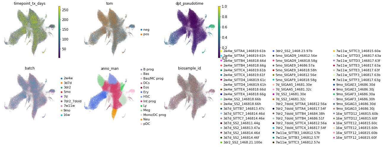
The preprocess single-cell landscape is batch-correted and cell type annotated.

sc.pl.umap(adata_full, 
           color=['timepoint_tx_days', 'tom', 'dpt_pseudotime',
                         'batch',  'anno_man', 'biosample_id', ], 
           ncols=3, wspace=0.3)

filtering Tom+ cells

For this particular data, the newly generated cells are labeled with fluorensence. We thus filtered Tomato-positive (Tom+) cells and count the number of all the Tom+ cells in the bone marrow. At each time point, we sequenced and FACS-counted cells from several mouse.

# select positive cells and saved under data
adata = adata_full[adata_full.obs['tom'] == 'pos'].copy()
adata.write_h5ad('data/tom_pos.h5ad')

Important !!!

To train the model, you need to placed the processed data under data.

1. Attaching population size measurement

One of the main innovations of pseudodyanmics+ is the use of population/tissue size measurement that comes from additional experiment, considering single-cell experiment has the issue of limiting capacity and sampling bias.

However, for dataset that without tissue size measurement, we can go back to sequenced cell number in the sc library. The parameters inferred in this manner may fail to reflect the absolute tissue growth and flux transiting between cell state.

The population info is stored as a dictionary and saved in adata.uns['pop']. The pop dictionary must contain the following keys:

• 't' : the real experiment time point when the cells are counted and sequenced (assume on the same day)

• 'mean' : the mean cell number of different experimental repeats for each time point

• 'std' : the standard derivation of different experimental repeats

• 'n_lib' : the number of repeats

For example, a single cell data with 3 time points (say day0, day4, day10) and 3 repeats each time looks like this:

    adata.uns['pop'] = {
        "t" = np.array([0, 4, 10]),
        "mean" = np.array([mean_d0, mean_d4, mean_d10]),
        "var" = np.array([var_d0, var_d4, var_d10]),
        "std" = np.array([std_d0, std_d4, std_d10]),
        "n_lib" = np.array([3, 3, 3])
    }

adata = sc.read_h5ad('data/tom_pos.h5ad')
adata

AnnData object with n_obs × n_vars = 49390 × 4814
    obs: 'n_genes', 'n_counts', 'mt_count', 'mt_frac', 'doublet_scores', 'predicted_doublets', 'xist_logn', 'Ygene_logn', 'xist_bin', 'Ygene_bin', 'sex_adata', 'biosample_id', 'cellid', 'RBG', 'SLXid', 'index', '10xsample_description', 'sex_mixed', 'sex_meta', 'mouse_id', 'sortedcells', 'expected_cells_10x', 'cellranger_cellsfound', 'chemistry', 'tom', 'expdate', 'batch', 'timepoint_tx_days', 'start_age', 'sample_id', 'countfile', 'S_score', 'G2M_score', 'phase', 'leiden', 'SLX', 'plate_sorted', 'plate_rearranged', 'well_sorted', 'well_rearranged', 'set_index', 'CI_index', 'mouse_platelabel', 'sort_method', 'sample.name', 'population', 'sex', 'countfolder', 'batch_plate_sorted', 'data_type', 'sex_combined', 'longname', 'anno_man', 'leiden_DM', 'HSCscore', 'nn_HSCscore', 'isroot', 'dpt_pseudotime', 'leiden_orig', 'logk', 'net_prolif', 'log10SR', 'log_density_at_E3', 'log_density_at_E7', 'log_density_at_E12', 'log_density_at_E12_clip', 'log_density_at_E3_clip', 'log_density_at_E7_clip', 'log_density_at_E27', 'log_density_at_E27_clip', 'log_density_at_E49', 'log_density_at_E49_clip', 'log_density_at_E76', 'log_density_at_E76_clip', 'log_density_at_E112', 'log_density_at_E112_clip', 'log_density_at_E161', 'log_density_at_E161_clip', 'log_density_at_E269', 'log_density_at_E269_clip', 'pseudo_bulk', 'rs50', 'split', 'fine_anno'
    var: 'symbol', 'gene_ids-10x', 'feature_types-10x', 'genome-10x', 'n_counts-10x', 'highly_variable-10x', 'means-10x', 'dispersions-10x', 'dispersions_norm-10x', 'gene_removed-10x', 'mean-10x', 'std-10x', 'geneid-SS2', 'chromosome-SS2', 'is_mito-SS2', 'highly_variable', 'mean', 'std'
    uns: 'DM', 'DM_EigenValues', 'anno_man_colors', 'biosample_id_colors', 'data_type_colors', 'density_predictor', 'diffmap_evals', 'fine_anno_colors', 'iroot', 'isroot_colors', 'leiden', 'leiden_DM_colors', 'leiden_DM_sizes', 'leiden_colors', 'leiden_sizes', 'neighbors', 'original_pop', 'paga', 'pagaDM', 'pagaPCA', 'pca', 'phase_colors', 'pop', 'predicted_doublets_colors', 'pseudo_bulk', 'pseudo_bulk_settings', 'rank_genes_groups', 'rs50', 'umap_init_pos', 'umap_init_pos_DM'
    obsm: 'DM_EigenVectors', 'DM_scaled', 'Delta_DM', 'TIGON_u', 'X_diffmap', 'X_pca', 'X_pca_harmony', 'X_pca_scaled', 'X_umap', 'X_umap_2d', 'X_umap_3d', 'X_umap_DM_2d', 'X_umap_DM_3d', 'mellon_u', 'surrogate_u'
    varm: 'PCs'
    obsp: 'DM_Kernel', 'DM_Similarity', 'DM_connectivities', 'DM_distances', 'connectivities', 'distances'

load FACS data

Here we are loading the FACS experiment data. The BM cells of the same mouse are sorted for tomato positive and count total cell number before sending for sequencing.

pop_df = pd.read_csv("data/tompos/model_input_tompos.csv")
pop_df.head()

	biosample_id	0	1	2	3	4	5	6	7	8	...	20	24	25	26	28	sc_ncells_filt	flow_total	start_age	time	sc_ncells_total
0	2w4w_SITTC4_146819.61b	42	16	8	5	15	7	3	19	28	...	0	0	0	0	0	157	634.907992	young	27	161
1	2w4w_SITTC4_146819.61f	184	122	103	109	118	97	73	149	146	...	4	11	2	5	2	1304	2320.519107	young	27	1357
2	2w4w_SITTD4_146819.61c	257	122	107	76	116	120	78	175	161	...	7	4	3	2	1	1422	3535.791587	young	27	1449
3	2w4w_SITTD4_146819.61h	98	61	42	45	42	26	28	52	76	...	2	2	0	1	0	547	895.421264	young	27	563
4	2w4w_SITTE4_146818.66d	35	10	10	9	6	16	4	19	16	...	0	0	0	1	0	137	456.845376	young	12	143

5 rows × 26 columns

We summarize the total cell number over different mouse for each time point

pop_by_time = pop_df.groupby("time").agg({"flow_total":["mean", "std","count"], "sc_ncells_filt":["mean", "std"]})
pop_by_time

	flow_total			sc_ncells_filt
	mean	std	count	mean	std
time
3	147.000000	45.745674	4	101.00	36.487441
7	388.645708	254.329995	6	150.50	69.856281
12	576.692900	169.724308	4	155.25	106.859331
27	1846.659988	1347.949806	4	857.50	606.941238
49	3123.277705	2110.007646	4	1143.00	813.058833
76	8233.932637	446.605979	2	2678.00	560.028571
112	13949.548025	6560.283561	4	3003.25	1733.310392
161	4941.850616	3795.978265	4	1854.25	1635.804262
269	41722.985970	1788.570460	2	4320.75	1446.069241

import matplotlib.pyplot as plt


def plot_mean_std(col_name, ax):
    time_points = pop_by_time.index
    mean_values = pop_by_time[(col_name, 'mean')]
    std_values = pop_by_time[(col_name, 'std')]

    ax.plot(range(len(time_points)), mean_values, marker='o', label=col_name)
    ax.fill_between(range(len(time_points)), 
                    mean_values - std_values, 
                    mean_values + std_values, 
                    alpha=0.3, color='gray', label=col_name+"_error")
    ax.set_xticks(range(len(time_points)))
    ax.set_xticklabels(time_points)

fig = plt.figure(dpi=80, figsize=(6, 3))
ax = fig.gca()
plot_mean_std('flow_total', ax=ax)

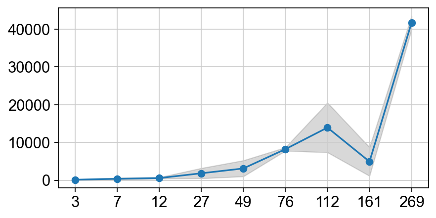
Here we found that the measurment at Day 161 seems to be an outlier. We do the following correction :

• we estimate the average growth rate from Day112 to Day269 with \( N_t = N_0 * e^{g \Delta t}\)

• next we impute the mean pop size at Day161 with the average growth rate

time_points = pop_by_time.index
mean_values = pop_by_time[('flow_total', 'mean')].values
g = np.log(mean_values[-1]  / mean_values[-3]) / (time_points[-1] - time_points[-3]) 
print(f'the estimated mean g is {g:.5f}')

impute_Day161 = np.exp(g*(time_points[-2] - time_points[-3]) ) * mean_values[-3]
print(f'the imputed mean pop size is {impute_Day161:.2f}')

# replace the mean value
mean_values[-2] = impute_Day161

the estimated mean g is 0.00698
the imputed mean pop size is 19636.45

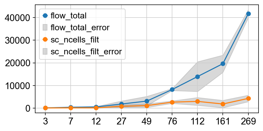
fig = plt.figure(dpi=80, figsize=(6, 3))
ax = fig.gca()
plot_mean_std('flow_total', ax)
plot_mean_std('sc_ncells_filt', ax)
ax.legend()

<matplotlib.legend.Legend at 0x3264a7f50>

# assign to uns['pop']

adata.uns['pop'] = {
    't' : time_points.to_numpy(),
    'mean' : mean_values,
    'var' : pop_by_time[('flow_total', 'std')].values ** 2,  # variance per timepoint
    'std' : pop_by_time[('flow_total', 'std')].values,
    'n_lib' : pop_by_time[('flow_total', 'count')].values
}

adata.uns['pop']

2. rename Timepoint Key

We use a unique obs key timepoint_tx_days to store the timepoint.

if 'timepoint_tx_days' not in adata.obs_keys():
    adata.obs['timepoint_tx_days'] = adata.obs['day'].astype(int) # example

check if the time point from the pop info match with that in the sequencing data

adata.obs['timepoint_tx_days'].isin(adata.uns['pop']['t']).all()

True

3. Compute diffusion map (DM)

The example dataset has pre-computed diffusion maps. For reproducibility, plesae keep the original diffusion map and pseudotime.
Here, for demonstration, we show two popular methods of getting DM cooridnates and pseudotime.

• scanpy diffusion map and dpt_psuedotime

• palantir diffusion map and palantir pseudotime

adata

AnnData object with n_obs × n_vars = 49390 × 4814
    obs: 'n_genes', 'n_counts', 'mt_count', 'mt_frac', 'doublet_scores', 'predicted_doublets', 'xist_logn', 'Ygene_logn', 'xist_bin', 'Ygene_bin', 'sex_adata', 'biosample_id', 'cellid', 'RBG', 'SLXid', 'index', '10xsample_description', 'sex_mixed', 'sex_meta', 'mouse_id', 'sortedcells', 'expected_cells_10x', 'cellranger_cellsfound', 'chemistry', 'tom', 'expdate', 'batch', 'timepoint_tx_days', 'start_age', 'sample_id', 'countfile', 'S_score', 'G2M_score', 'phase', 'leiden', 'SLX', 'plate_sorted', 'plate_rearranged', 'well_sorted', 'well_rearranged', 'set_index', 'CI_index', 'mouse_platelabel', 'sort_method', 'sample.name', 'population', 'sex', 'countfolder', 'batch_plate_sorted', 'data_type', 'sex_combined', 'longname', 'anno_man', 'leiden_DM', 'HSCscore', 'nn_HSCscore', 'isroot', 'dpt_pseudotime', 'leiden_orig', 'logk', 'net_prolif', 'log10SR', 'log_density_at_E3', 'log_density_at_E7', 'log_density_at_E12', 'log_density_at_E12_clip', 'log_density_at_E3_clip', 'log_density_at_E7_clip', 'log_density_at_E27', 'log_density_at_E27_clip', 'log_density_at_E49', 'log_density_at_E49_clip', 'log_density_at_E76', 'log_density_at_E76_clip', 'log_density_at_E112', 'log_density_at_E112_clip', 'log_density_at_E161', 'log_density_at_E161_clip', 'log_density_at_E269', 'log_density_at_E269_clip', 'pseudo_bulk', 'rs50', 'split', 'fine_anno'
    var: 'symbol', 'gene_ids-10x', 'feature_types-10x', 'genome-10x', 'n_counts-10x', 'highly_variable-10x', 'means-10x', 'dispersions-10x', 'dispersions_norm-10x', 'gene_removed-10x', 'mean-10x', 'std-10x', 'geneid-SS2', 'chromosome-SS2', 'is_mito-SS2', 'highly_variable', 'mean', 'std'
    uns: 'DM', 'DM_EigenValues', 'anno_man_colors', 'biosample_id_colors', 'data_type_colors', 'density_predictor', 'diffmap_evals', 'fine_anno_colors', 'iroot', 'isroot_colors', 'leiden', 'leiden_DM_colors', 'leiden_DM_sizes', 'leiden_colors', 'leiden_sizes', 'neighbors', 'original_pop', 'paga', 'pagaDM', 'pagaPCA', 'pca', 'phase_colors', 'pop', 'predicted_doublets_colors', 'pseudo_bulk', 'pseudo_bulk_settings', 'rank_genes_groups', 'rs50', 'umap_init_pos', 'umap_init_pos_DM'
    obsm: 'DM_EigenVectors', 'DM_scaled', 'Delta_DM', 'TIGON_u', 'X_diffmap', 'X_pca', 'X_pca_harmony', 'X_pca_scaled', 'X_umap', 'X_umap_2d', 'X_umap_3d', 'X_umap_DM_2d', 'X_umap_DM_3d', 'mellon_u', 'surrogate_u'
    varm: 'PCs'
    obsp: 'DM_Kernel', 'DM_Similarity', 'DM_connectivities', 'DM_distances', 'connectivities', 'distances'

if 'X_diffmap' not in adata.obsm_keys():
    # use batch corrected cell representation like Harmonied PC or SCVI latent
    sc.pp.neighbors(adata, n_pcs=30, use_rep='X_pca_harmony') 
    sc.tl.diffmap(adata, n_comps=10)

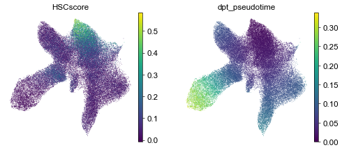
adata.uns['iroot']= np.argmin(adata.obs['HSCscore'].values)
sc.tl.dpt(adata)

sc.pl.umap(adata, color=['HSCscore', 'dpt_pseudotime'])

# next we scaled the diffusion map to 0-1.
DM = adata.obsm['X_diffmap']
DM_min = DM.min(axis=0,keepdims=True)
DM_range = DM.max(axis=0,keepdims=True) - DM_min
DM_scaled = (DM - DM_min)/DM_range

Use palantir to compute DM

import palantir
dm_res = palantir.utils.run_diffusion_maps(adata, pca_key='X_pca_harmony')
ms_data = palantir.utils.determine_multiscale_space(adata)

print(f"shape of palantir DM : {adata.obsm['DM_EigenVectors'].shape} and scaled DM : {adata.obsm['DM_EigenVectors_multiscaled'].shape} ")

4. Sample local cell state changes in diffusion map

Pseudodynamics+ can make use of the local cell state changes in diffusion map to assists learning velocity, inspired by TrajectoryNet by Tong et. al.. This state changes is defined as \(\Delta x = \sum_{i \in N(x)} \frac{w_{i,x}}{w_{i,x} + \sum_{j \in N(x)} w_{i,j}} \Delta x_i\) ,Here we provdie two ways of sampling this local state transition:

• by default we rely on KNN and pseudotime with \(w_{i,j}\) denoting the connectivities in KNN.

• alternatively, when a transition matrix is provided, e.g. cellrank. The \(w_{i,j}\) denote the probability of transitioning from \(i\) to \(j\).

delta_DM , neighbors = pdp.tl.sample_deltax(adata, xkey='DM_scaled', pseudotimekey='dpt_pseudotime', repeat=10)
delta_DM_ay = np.stack(delta_DM)

print(delta_DM_ay.shape)
adata.obsm['Delta_DM'] = delta_DM_ay.mean(axis=-1) # use the averaged ∆DM

(49390, 10, 30)

5. train test split

def train_test_split_adata(adata,  leaveout=None, val_size=0.1, test_size=0.1, timepoint_key='timepoint_tx_days'):

    obs = adata.obs
    val_test_cbs = obs.query(f"`{timepoint_key}` not in @leaveout").sample(frac=0.2).index
    test_cb = np.random.choice(val_test_cbs, size=len(val_test_cbs)//2,replace=False)

    split_mapper = {cb:'test' for cb in test_cb}
    val_cbs = {cb:'val' for cb in val_test_cbs if cb not in test_cb}
    train_cbs = {cb:'train' for cb in adata.obs_names if cb not in val_test_cbs}

    split_mapper.update(val_cbs)
    split_mapper.update(train_cbs)

    return adata.obs.index.map(split_mapper)

adata.obs['split'] = train_test_split_adata(adata, leaveout=[3])

adata.write_h5ad("data/tom_pos.h5ad")

What’s next

• Estimate single-cell density at observed time point (optional).

• set up training configuration